Lab 1 : Signal Filtering

Platform: Software Defined Radios.

Resources needed: 2 x USRP B210s

Short Description: Implement signal filtering and noise reduction techniques using Software Defined Radios

Detailed Description: GNU Radio is used to implement low-pass, high-pass, band-pass, and band-stop filters to clean up a received signal. Varying degrees of artificial noise can be added to the signal and the constructed filters will be used to improve the clarity of the signal.

In this lab, we will be using Python. Follow the steps below to start this experiment:

1. Open Visual Studio Code and make sure you have the following extensions installed: Python, Pylance, Python Environment Manager, GNURadio Integration, GNURadio Development Pack

2. Once you have these extensions added, you will open a new file in VS and title it ‘lowpassfilterExperiment.py’

3. Add this block of code to the file you just created:

   import numpy as np
   import matplotlib.pyplot as plt
   
   H = np.hstack((np.zeros(20), np.arange(10)/10, np.zeros(20)))
   w = np.linspace(-0.5, 0.5, 50)
   plt.plot(w, H, '.-')
   plt.show()
   
   h = np.fft.ifftshift(np.fft.ifft(np.fft.ifftshift(H)))
   plt.plot(np.real(h))
   plt.plot(np.imag(h))
   plt.legend(['real','imag'], loc=1)
   plt.show()
   

Save this file, but before running it, make sure all necessary libraries are downloaded (you will have to install matplotlib or alternative plotting library)

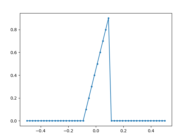
You should see the following output after running this file:

align:

center

alt:

Low-pass time response

name:

img-lowpass-time

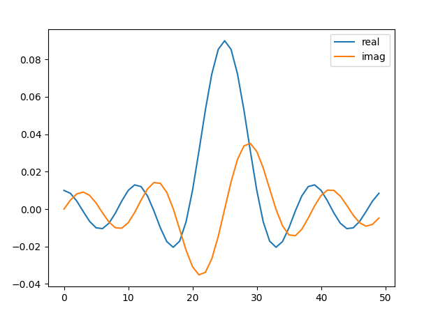
The first image represents the filter’s impulse response in the time domain while the second image shows the responses with real taps and complex taps.

You should see the following output after running this file:

align:

center

alt:

Low-pass frequency / impulse

name:

img-lowpass-freq

1. Now create a new file and title it ‘lowpasstohighpass’

2. Add the following code to this file:

   import numpy as np
   from gnuradio import gr
   from gnuradio import uhd
   from gnuradio import blocks
   import time
   import matplotlib.pyplot as plt
   
   class top_block(gr.top_block):
       def __init__(self):
           gr.top_block.__init__(self, "Top Block")
   
           # Parameters
           samp_rate = 1e6
           center_freq = 3586.98e6
           gain = 50
   
           # USRP Source
           self.usrp_source = uhd.usrp_source(
               ",".join(("", "")),
               uhd.stream_args(
                   cpu_format="fc32",
                   channels=[0],
               ),
           )
           self.usrp_source.set_samp_rate(samp_rate)
           self.usrp_source.set_center_freq(center_freq, 0)
           self.usrp_source.set_gain(gain, 0)
   
           self.vector_sink = blocks.vector_sink_c()
   
           self.connect((self.usrp_source, 0), (self.vector_sink, 0))
   
       def get_data(self):
           return self.vector_sink.data()
   
   # Create and run the flowgraph
   tb = top_block()
   tb.start()
   print("Collecting samples...")
   time.sleep(1)
   tb.stop()
   tb.wait()
   print("Sample collection complete.")
   
   data = tb.get_data()
   plt.scatter(np.real(data), np.imag(data))
   plt.title('Received Signal')
   plt.xlabel('Real Part')
   plt.ylabel('Imaginary Part')
   plt.savefig("gnuexampleoutput.png", dpi=150)
   

3. This file will build a filter using GNURadio, a commonly used SDR platform. Here, several modules are defined and connected together in a flowgraph. Running the flowgraph in GNURadio will simulate real time frequency responses and demonstrate the behavior of a signal as it passes through the filter.

4. Run this file a couple times while changing the ‘samp_rate’ and ‘center_freq’ values in the file. See if you can develop high-pass, band-pass, and band-stop responses as well as low-pass.