Sampling Theory and Application

Basics of Sampling

Introduction

Sampling is the process of capturing values at certain moments in time, usually in a set interval of time in order to ensure an accurate sampling size and dataset. The sample period is the recorded value of a function at regular intervals of seconds while the sample rate is the exact inverse of the sample period, or the number of samples taken per second (the frequency of sampling).

Understanding how Sampling Theory works

Using sampling and a process called quantization, continuous-time analog signals can be converted to discrete-time digital signals. Sampling is defined as the conversion between continuous and discrete-time signals. This is done by taking samples of the continuous-time signal at discrete-time points. Quantization comes in as the process that converts the amplitude of the sample digitally. The reverse can be done, converting a discrete-time signal to a continuous-time signal which is called reconstruction. One important sampling method is uniform sampling, which is the process of capturing the most widely used sampling.

Uniform Sampling

Also called periodic sampling, this method specifies the sampling interval as a constant number to take samples of the continuous-time signal every specified number of seconds. This process is most easily shown in the frequency domain. First, the Fourier transform is taken of the signal’s function and then the multiplication of that function in the time domain leads to the occurrence of convolution in the frequency domain.

Nyquist Sampling

The theorem proposed by a physicist by name of Harry Nyquist stated that a real signal can be reconstructed with no errors from uniform sampling at a rate of R > 2B samples/second (the signal being bandlimited to B Hz). However, the undersampling of a signal results in a lack of complete information about the spectrum and does not allow the signal to be recovered any longer.

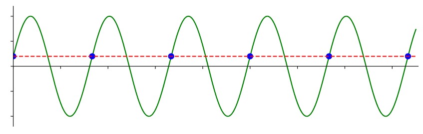
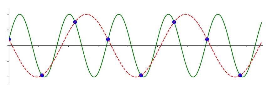
Here, samples of a signal are taken at a rate of f and 1.5f, showing the ambiguity that develops as a result. This means that signals cannot be differentiated from each other or reconsructed at all because the sampling does not fit the signal being captured. This is why sampling must always be taken at twice the frequency of the signal. More accurately, the sample rate must be twice the frequency of the signal’s maximum frequency component. Not sampling fast enough leads to aliasing, undersampling as a result of frequency components overlapping, which is highly undesirable. The occurrence of this phenomena distorts the signal and makes it incredibly difficult to recover at the signal receiver.

Decimation is the process of lowering the sample rate, which is desirable in real world applications because of lower storage and computation requirements. This process is achieved by taking only every Dth sample where D is the decimation rate. Decimation can be set up using a lowpass anti-aliasing filter and a downsampler. Interpolation is the process of increasing the sampling rate. This is done by injecting new signals in between successive values of signal. Interpolation can be set up using the reverse of Decimation, having an upsampler in connection with a lowpass filter.

Since most modern applications like WiFi, Bluetooth, LTE, and others use radio frequency ranges from 100 MHz to 6 Hz, the carrier for these signals will often lie in this range. Frequencies for radar and satellite communications are now also used in 5G mmWave applications which falls in a range of 24 to 29 GHz. Essentially, when a signal is received, it is stored as complex values and being sampled at a given rate that the SDR is picking up. This frequency rate is different from the carrier rate (which is the frequency on which the signal is transmitted). In short, the carrier frequency defines the signal that is being transmitted while the sampling of this signal is occurring at twice the frequency of the carrier (to avoid resulting ambiguity as mentioned above).

This is a summary of the sampling process and only grazes the many components involved. In the remainder of this module, you will learn how key concepts of Convolution and Correlation round out signal processing and analyzation.